This is continuing from the previous post, where I discussed how we convert data collected by ATLAS into usable objects. Here I explain the steps to get a Physics result.

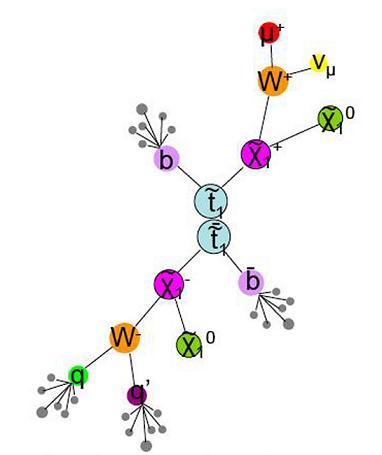
I can now use our data sample to prove/disprove the predictions of Supersymmetry (SUSY), string theory or what have you. What steps do I follow? Well, I have to understand the predictions of this theory; is it saying that there will be multiple muons in an event or there will be only one very energetic jet in the event, etc? For instance, the accompanying figure shows the production and decay of SUSY particles, which lead to events with many energetic jets, a muon, and particles that escape the detector without leaving a trace (missing energy), like X₁.

If the signature is unique, then my life is considerably simpler; essentially, I will write some software to go through each event and pick out those that match the prediction (you can think of this as finding the proverbial (metal) needle in a haystack). If the signal I am searching for is not very unique, then I have to be much cleverer (think of this as looking for a fat, wooden needle in a haystack).

First, I have to decide the selection criteria, e.g., I want one muon with momentum greater than, say, 100 GeV/c, or one electron and exactly two jets, etc. Once I’ve decided the selection criteria, I cannot change them, and have to accept the results, whatever they may be. Otherwise, there is a very real danger of biasing the result. To decide these selection criteria, I may look at simulation, i.e., fake data, and/or sacrifice a small portion of real data to do my studies on. With these criteria, I could have a non-zero number of candidate events, or zero events.

In either case, I have to estimate how many events I expect to see due to garden-variety physics effects, which can occur as much as a million or a billion times more frequently, and may produce a similar signature; this is called background. This can happen because our reconstruction software could mis-identify a pion as a muon, or make a wrong measurement of an electron’s energy, or if we produce enough of these garden-variety events a few of them (out in the “tails”) may look like new physics. So I have to think of all the standard processes that can mimic what I am searching for. One way to do this is to run my analysis software on simulated events; since we know what a garden-variety process looks like, we generate tons of fake data and see if some events look like the new effect that I am looking for. I can also use “real” data, and by applying a different set of selection criteria, come up with what we call “data driven background estimate”. If the background estimate is much less than the number of candidate signal events, excitement mounts, and the result pops up on the collaboration’s radar screen.

There is usually a trade-off between increasing the efficiency of finding signal events and reducing background. If you use loose selection criteria, you expect to find more signal events, i.e., increase in efficiency, but also more background. Since the background can overwhelm the signal, one has to be careful. Conversely, if you choose very strict criteria, you could have zero background, but also zero signal efficiency – not very useful!!

There is one more thing that I need to do, which sometimes can take a while, and for which there is definitely no standard prescription. I need to determine systematic uncertainties, i.e., an error estimate for my methodology, on both the signal efficiency, and on the background estimate. For instance, if I use a meter-scale to measure the length of a table, how do I know the meter-scale is correct? I have to quantify the correctness of the meter-scale. A result in our field has to have systematic uncertainties otherwise it is meaningless. This step is usually a source of lot of arguments. For instance, in the paper mentioned in Part 1, we say that there is a systematic uncertainty of 6.6% (see section 6). Depending on whether this is smaller (larger) than the statistical uncertainty, we say that the result is statistics (systematics) limited. In the first case, adding more data is necessary, and in the second case, a better understanding is needed. At times, one can have a statistical fluctuation that disappears by adding more data; conversely, many results go by the wayside because of people not understanding systematic effects.

Since there is no fixed recipe to do analysis, I can sometimes run into obstacles, or my results may look “strange”; I then have to step back and think about what is going on. After I get some preliminary results I have to convince my colleagues that they are valid; this involves giving regular progress reports within the analysis group. This is followed by a detailed note, which is reviewed by an internal committee appointed by the experiment’s Publication Committee and/or the Physics Coordinator. If I pass this hurdle, the note is released to the entire collaboration for further review. All along this process, people ask me to do all sorts of checks, or tell me that I am completely wrong, or whatever. Given that every physicist thinks that he/she is smarter than the next, this process can be cantankerous at times, since I have to respond to and satisfy each and every comment. Once the experiment’s leader signs off on the paper, we submit it to a peer-reviewed journal, where the external referee(s) can make you jump through hoops; sometimes their objections are valid, sometimes not. I have been on both sides of this process. Needless to say, as a referee my objections are always valid!!

Depending on the complexity of the analysis, the time from the start to finish can be anywhere from a few months to a year or more (causing a few more grey hair, or in my case a few less hair). The two papers that I mentioned at the start of part 1 took about 1-2 years each. Luckily, I had collaborators and we divided up the work among ourselves, so I could work on both of them in parallel.